Statistical Analysis
Here is some additional analysis of the data set.
First, the same loading and cleaning method was used.
Does the average number of crash events differs across months?
To investigate potential seasonal trends in aviation safety, we selected data from Northern Hemisphere and plot the accident per month. We then performed a One-Way ANOVA to determine if the average number of airplane crashes differs significantly across the months.
The ANOVA results yielded a p-value of 0.039, which was below the 0.05 significance level. Although, the average number of crashes per month is small, so even a few events can create “significant” differences.
airplane_north = df_map |>
  filter(aboard > 0, !is.na(fatalities))|>
   filter(Latitude> 0)|>
  mutate(
    survival_rate = (aboard - fatalities) / aboard,
    month_num     = month(date),
    season = case_when(
      month_num %in% c(12, 1, 2)  ~ "Winter",
      month_num %in% c(3, 4, 5)   ~ "Spring",
      month_num %in% c(6, 7, 8)   ~ "Summer",
      month_num %in% c(9, 10, 11) ~ "Fall"
    )
  ) |>
  filter(!is.na(season)) |>
  mutate(season = fct_relevel(season, "Spring", "Summer", "Fall", "Winter"))

cat("=== ANOVA result ===\n")
## === ANOVA result ===airplane_north |>
# Count crashes per year/season combo
count(year, month, name = "crash_count")|>
# ANOVA
aov(crash_count ~ factor(month), data = _) |>
summary()## Df Sum Sq Mean Sq F value Pr(>F)
## factor(month) 11 60.2 5.470 1.873 0.0393 *
## Residuals 923 2695.8 2.921
## ---
## Signif. codes: 0 '***' 0.001 '**' 0.01 '*' 0.05 '.' 0.1 ' ' 1# ---- plot ----
airplane_north |>
count(year, month, name = "crash_count")|>
group_by(month) |>
summarise(
mean_crashes = mean(crash_count),
se = sd(crash_count) / sqrt(n())
) |>
ggplot(aes(x = month, y = mean_crashes)) +
scale_x_continuous(breaks = 1:12) +
geom_col(fill = "steelblue",show.legend = FALSE) +
geom_errorbar(aes(ymin = mean_crashes - se,
ymax = mean_crashes + se),
width = 0.15) +
labs(
title = "Average Airplane Crashes in Northern Hemisphere per Month",
x = "Month",
y = "Average Crash Count"
) +
theme_minimal()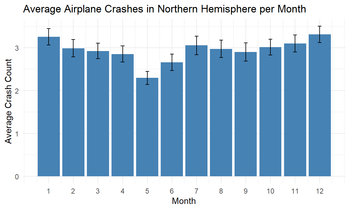
We also test for the differences of fatality rate across months. BUt there is no significant evidence suggested a monthly difference of fatality rate.
cat("=== ANOVA result ===\n")## === ANOVA result ===airplane_north|>
##ANOVA
aov(survival_rate ~ factor(month), data = _ )|>
summary()## Df Sum Sq Mean Sq F value Pr(>F)
## factor(month) 11 0.76 0.06933 0.675 0.764
## Residuals 2749 282.37 0.10272Is the fatality rate lower over time?
To evaluate the long-term trend in survivability, we plot the fatality rates per year. Statistical evidence confirmed that airplanes have become safer over time regarding rate of survival. Linear regression analysis revealed a statistically significant negative correlation between year and fatality rate (p < 0.001).
However, the low R-squared value (0.015) indicated that while the downward trend is consistent, the outcome of any individual crash is heavily influenced by situational factors other than just the time period, and the average fatality rate of a single year is still largely determined by random effect.
 airplane_df |>
  filter(aboard > 0, !is.na(fatalities)) |>
  mutate(fatality_rate = fatalities / aboard) |>
  group_by(year) |>
  summarise(mean_fatality_rate = mean(fatality_rate)) |>
  ggplot(aes(x = year, y = mean_fatality_rate)) +
  geom_point(color = "steelblue", alpha = 0.6) +
  geom_smooth(method = "lm", color = "red", fill = "pink",se = TRUE) +
   scale_x_continuous(breaks = seq(1910, 2010, by = 10)
  )+
  labs(
    title = "Trend in Airplane Fatality Rate Over Time",,
    x = "Year",
    y = "Average Fatality Rate"
  ) +
  theme_minimal()
## `geom_smooth()` using formula = 'y ~ x'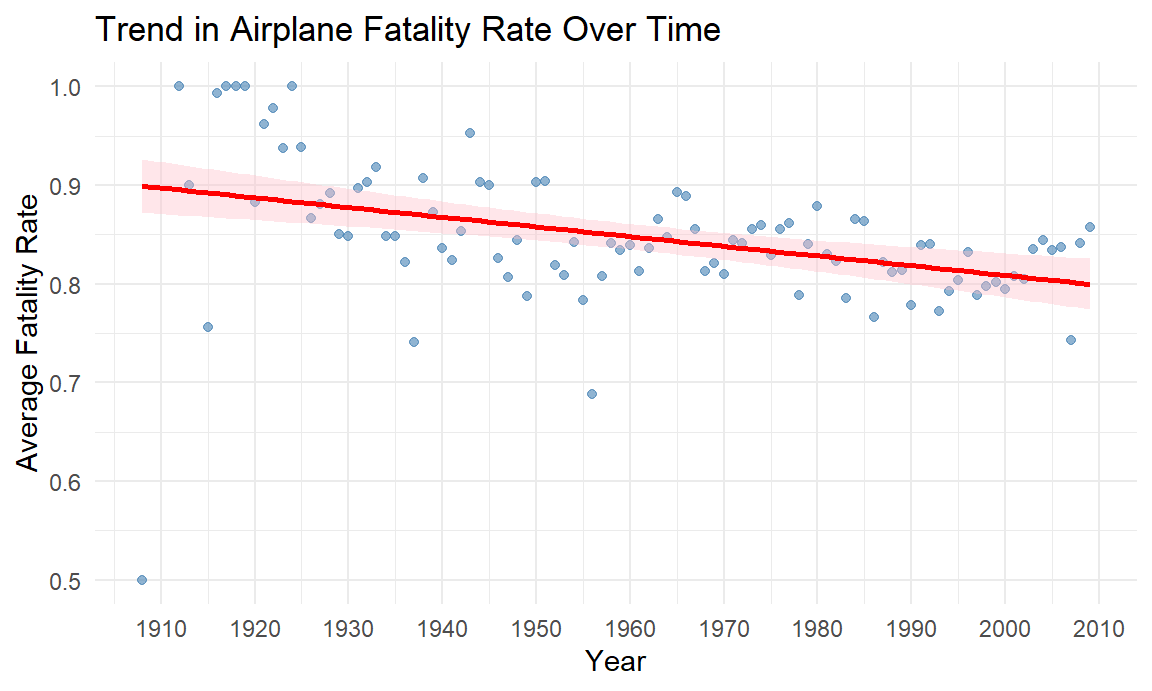
 airplane_df |>
  filter(aboard > 0, !is.na(fatalities)) |>
  mutate(fatality_rate = fatalities / aboard) |>
  group_by(year) |>
  summarise(mean_fatality_rate = mean(fatality_rate))|>
 lm(mean_fatality_rate ~ year, data = _)|> summary()
##
## Call:
## lm(formula = mean_fatality_rate ~ year, data = summarise(group_by(mutate(filter(airplane_df,
## aboard > 0, !is.na(fatalities)), fatality_rate = fatalities/aboard),
## year), mean_fatality_rate = mean(fatality_rate)))
##
## Residuals:
## Min 1Q Median 3Q Max
## -0.39929 -0.02716 0.00041 0.03606 0.11644
##
## Coefficients:
## Estimate Std. Error t value Pr(>|t|)
## (Intercept) 2.7754226 0.4526676 6.131 1.93e-08 ***
## year -0.0009833 0.0002309 -4.259 4.79e-05 ***
## ---
## Signif. codes: 0 '***' 0.001 '**' 0.01 '*' 0.05 '.' 0.1 ' ' 1
##
## Residual standard error: 0.0649 on 96 degrees of freedom
## Multiple R-squared: 0.1589, Adjusted R-squared: 0.1502
## F-statistic: 18.14 on 1 and 96 DF, p-value: 4.79e-05Are the number of crash events higher or lower over the years?
To describe the historical trend of aviation safety, we aggregated the total number of crashes per year. We then fitted a simple linear regression model and Loess model to determine if there was a statistically significant linear increase or decrease in crash frequency over the recorded time period (1908–2009). With a medium fitted model, the linear regression analysis revealed a statistically significant upward trend.But this failed to accurately describe the crash events overtime, LOESS could reveal more specific fluctuations and details in history.
crashes_by_year = airplane_df |>
  count(year, name = "total_crashes")

ggplot(crashes_by_year, aes(x = year, y = total_crashes)) +
  geom_point(color = "steelblue", alpha = 0.6) +
  geom_smooth(method = "lm", color = "red", fill = "pink", se = TRUE, span = 0.2)+
  geom_smooth(method = "loess", color = "royalblue", fill = "lightblue", se = TRUE, span = 0.2) +
  scale_x_continuous(breaks = seq(1910, 2010, by = 10)
  ) +
  labs(
    title = "Trend of Total Airplane Crashes per Year",
    subtitle = "Red: Linear Trend | Blue: LOESS Trend",
    x = "Year",
    y = "Total Number of Crashes"
  ) +
  theme_minimal()
## `geom_smooth()` using formula = 'y ~ x'
## `geom_smooth()` using formula = 'y ~ x'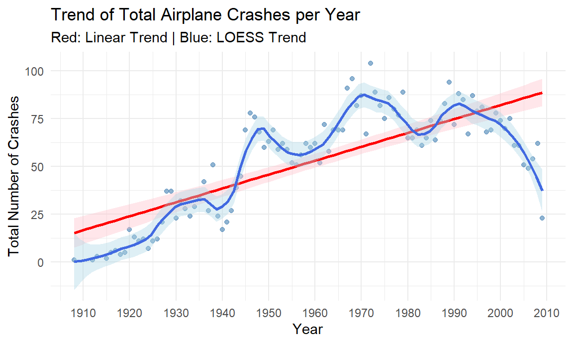
fit_count_linear = lm(total_crashes ~ year, data = crashes_by_year)
summary(fit_count_linear)
##
## Call:
## lm(formula = total_crashes ~ year, data = crashes_by_year)
##
## Residuals:
## Min 1Q Median 3Q Max
## -65.727 -12.685 -0.066 11.661 42.168
##
## Coefficients:
## Estimate Std. Error t value Pr(>|t|)
## (Intercept) -1.372e+03 1.258e+02 -10.90 <2e-16 ***
## year 7.269e-01 6.415e-02 11.33 <2e-16 ***
## ---
## Signif. codes: 0 '***' 0.001 '**' 0.01 '*' 0.05 '.' 0.1 ' ' 1
##
## Residual standard error: 18.03 on 96 degrees of freedom
## Multiple R-squared: 0.5722, Adjusted R-squared: 0.5677
## F-statistic: 128.4 on 1 and 96 DF, p-value: < 2.2e-16The visual comparison demonstrated the limitations of the linear model. The linear fit failed to capture the mid-century rise and the late-century decline in crashes, resulting in high systematic error. The LOESS model provides the superior fit account for historical fluctuations and recent down trend.
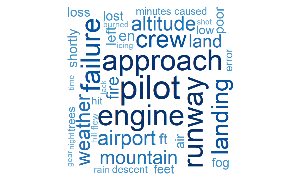
What could be the causes?
To see the causes and recurring themes of aviation incidents, we performed text mining on the crash summary descriptions. After tokenizing the text and removing common stop words (e.g., ‘the’, ‘and’,“plane”,“crashed”) and numbers, we generated a Word Cloud.
word_counts = airplane_df |>
  filter(!is.na(summary)) |>
  select(date, summary) |>
  unnest_tokens(word, summary) |>
  anti_join(stop_words) |>
  filter(!str_detect(word, "^[0-9]"))  |>
  filter(word != "crashed", word != "plane", word !="aircraft", word != "flight")|>
  count(word, sort = TRUE)
## Joining with `by = join_by(word)`set.seed(1234)
wordcloud(
words = word_counts$word,
freq = word_counts$n,
min.freq = 10,
max.words = 100,
random.order = FALSE,
rot.per = 0.25,
colors = brewer.pal(9, "Blues")[5:9]
)